Image interpolation algorithms

Interpolation is a technique in which we use to estimate the approximate continuous value of a function. Image interpolation occurs when you resize or remap your image from one pixel to another. Image resizing is necessary when you need to increase or decrease the total number of pixels, whereas remapping can occur under a wider variety of scenarios, such as correcting for lens distortion, changing perspective, or rotating an image.

Interpolation algorithms can be divided into two groups: adaptive algorithms and non-adaptive algorithms. The adaptive algorithms change depending on the purpose of the interpolation, these algorithms are primarily designed to maximise artefact-free detail in enlarged photos, so some cannot be used to distort or rotate an image. Whereas the non-adaptive algorithms treat pixels equally, they use anywhere from \(0\) to \(256\) adjacent pixels when interpolating. The more adjacent pixels they include, the more accurate they become, but this comes at the expense of much longer processing time. These algorithms can be utilised for both distorting and resizing photos.

In this post, we will be covering the most common non-adaptive interpolation algorithms, which are the nearest neighbour, bilinear, and bicubic. They have advantages in simplicity and fast implementation.

1. Nearest neighbour interpolation

The nearest neighbour is the most basic and requires the least processing time of all the interpolation algorithms. With this method, we are just basically taking the pixels from the original image and making them bigger to form the scaled image. Let’s have a look at the example below.

Nearest neighbour interpolation

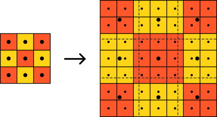
Figure 1. Nearest neighbour interpolation.

We have the big dots at the centre of the cells that represent the pixels in the original image. They are then stretched to the size of the scaled image and overlaid onto it. We also have the small dots in the scale image, which represent its pixels. These pixels then take the same value as the pixel represented by the closest big dot.

Below is a sample of C++ code for the nearest neighbour interpolation:

// The nearest neighbour interpolation
for (int destination_row = 0; destination_row < destination.rows; ++destination_row)
{
    for (int destination_column = 0; destination_column < destination.cols; ++destination_column)
    {
        int destination_index = destination_row * destination.cols + destination_column;
        int source_row = std::round(pixel_map[destination_index].row);
        int source_column = std::round(pixel_map[destination_index].column);
        int source_index = source_row * source.cols + source_column;
        for (int i = 0; i < number_of_channels; ++i)
        {
            // Assign to the closest pixel
            destination.data[destination_index * number_of_channels + i] = source.data[source_index * number_of_channels + i];
        }
    }
}

You can find the complete version of the code here.

2. Bilinear interpolation

With the bilinear interpolation, instead of making the pixels bigger to form the scaled image, it is blending the values of the pixels in the space between them. This algorithm considers the closest \(2\)x\(2\) neighbourhood pixels, which surround the unknown pixel. It then takes the weighted average of four pixels to estimate the interpolated value. One other thing to note here is that some pixels around the margins might not be surrounded by four pixels. The general way to deal with this is to create imaginary pixels past the margins of the image with the same value as the values of the margin pixels.

We can understand the bilinear interpolation by looking at the graphic below.

Bilinear interpolation algorithm

Figure 2. Bilinear interpolation algorithm.

In here, we have the green dot \(P\) that represents the point where we want to estimate the colour and the four red dots that represent the nearest pixels from the original image. In this example, \(P\) lies closest to \(Q_{12}\), so it is only appropriate that the colour of \(Q_{12}\) contributes more to the final colour of \(P\) than other \(Q\) pixels.

There are several equivalent ways to calculate the value of \(P\), and the easiest way would be to first calculate the value of the two blue dots \(R_2\) and \(R_1\). \(R_2\) is effectively a weighted average of \(Q_{12}\) and \(Q_{22}\), while the \(R_1\) is a weighted average of \(Q_{11}\) and \(Q_{21}\):

\[\begin{align} \left\lbrace \begin{array}{l} R_1 = \dfrac{x_2 - x}{x_2 - x_1}Q_{11} + \dfrac{x - x_1}{x_2 - x_1}Q_{21}\\ R_2 = \dfrac{x_2 - x}{x_2 - x_1}Q_{12} + \dfrac{x - x_1}{x_2 - x_1}Q_{22} \end{array} \right.. \tag{1} \end{align}\]

Once we have the values of \(R_1\) and \(R_2\), we can calculate the value of \(P\) as \begin{equation} P = \dfrac{y_2 - y}{y_2 - y_1}R_1 + \dfrac{y - y_1}{y_2 - y_1}R_2. \tag{2} \end{equation}

This method gives us noticeably smoother-looking images than the nearest neighbour interpolation.

You can find the complete version of the code here.

3. Bicubic interpolation

To understand the bicubic interpolation, we will start with the 1-dimensional case of the cubic interpolation. The cubic interpolation is a special case of the polynomial interpolation in which we fit a set of \(4\) given points into a third-degree polynomial. We have a third-degree polynomial function and its derivative as below:

\[\begin{align} \left\lbrace \begin{array}{l} f(x) = ax^3 + bx^2 + cx + d\\ f'(x) = 3ax^2 + 2bx + c \end{array} \right.. \tag{3} \end{align}\]

Let’s suppose we have the values of 4 points \(p_0\), \(p_1\), \(p_2\), and \(p_4\) at respectively \(x = -1\), \(x= 0\), \(x = 1\), \(x = 2\) are \(y_{-1}\), \(y_0\), \(y_1\), and \(y_2\).

Cubic interpolation

Figure 3. Cubic interpolation.

Without loss of generality, we can assume that we are interpolating between \(x = 0\) and \(x = 1\). We see that

\[\begin{align} \left\lbrace \begin{array}{l} f(0) = d\\ f(1) = a + b + c + d\\ f'(0) = c\\ f'(1) = 3a + 2b + c \end{array} \right.. \tag{4} \end{align}\]

Solving for the polynomial coefficients, we have

\[\begin{align} \left\lbrace \begin{array}{l} a = 2f(0) - 2f(1) + f'(0) + f'(1)\\ b = -3f(0) + 3f(1) - 2f'(0) - f'(1)\\ c = f'(0)\\ d = f(0) \end{array} \right.. \tag{5} \end{align}\]

Now let’s consider the four points around the region being estimated, and impose boundary conditions as

\[\begin{align} \left\lbrace \begin{array}{l} f(0) = y_0\\ f(1) = y_1\\ f'(0) = \dfrac{y_1 - y_{-1}}{2}\\ f'(1) = \dfrac{y_2 - y_0}{2} \end{array} \right.. \tag{6} \end{align}\]

By inserting \((6)\) into \((5)\), we get

\[\begin{align} \left\lbrace \begin{array}{l} a = -\dfrac{y_{-1}}{2} + \dfrac{3y_0}{2} - \dfrac{3y_1}{2} + \dfrac{y_2}{2}\\ b = y_{-1} - \dfrac{5y_0}{2} + 2y_1 - \dfrac{y_2}{2}\\ c = -\dfrac{y_{-1}}{2} + \dfrac{y_1}{2}\\ d = y_0 \end{array} \right.. \tag{7} \end{align}\]

Once we have the coefficients, we can interpolate \(f(x)\) for any point between \((0, y_0)\) and \((1, y_1)\). An important thing to note here is that cubic interpolation might sometimes end up slightly outside of the colour range (above unity or below \(0\)). In that case, our code must be able to clip these values.

The principle for the bicubic interpolation is pretty much the same as the cubic interpolation. The only difference is that you estimate a surface using \(16\) points (\(4\)x\(4\) rigid) rather than just a curve using 4 points. One simple way to do this is to first interpolate the columns and then interpolate the resulting rows.

Let’s have a look at the figure below, in which we run all three interpolation algorithms to scale up \(26\) times an image with the resolution of \(9\)x\(9\).

Image interpolation comparison

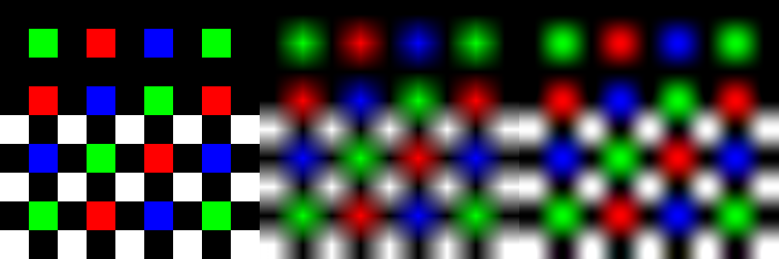
Figure 4. From left to right: nearest neighbour, bilinear, and bicubic.

As we can see here, the bilinear interpolation makes the colour transitions smooth, but we can notice unnatural vertical and horizontal bands in some places. The bicubic interpolation, on the other hand, produces a much sharper-looking image.

You can find the complete version of the code here.

References

← Previous Post Next Post →